
This is the rough draft. Nevertheless, copyright 2008 Lee Felshin.
A Computational Fluid Dynamics model is used to investigate the effect of tank geometry and baffling on the actual contact time (T10) in water tanks under various flow conditions. Preliminary results indicate that the actual T10s are much less than the theoretical plug flow
Many reactions take time to complete. In a continuous flow system, as opposed to batch system, mixed chemicals are given time to react in a detention tank. Calculating the contact time of a detention tank is difficult unless true plug flow is acheived.
In public water supply, chemical disinfection efficacy is related to the contact time. Until recently, small water supplies designed contact tanks based on two major simplifications, 15 minute contact time required and plug flow through the system. The former has been borne out as reasonable under most conditions of pathogen, pH, and temperature. The latter grossly overestimates the contact time of a tank.
Small water supply treatment plants are generally configured with a well pumping to a pressure tank (hydropneumatic tank) which feeds the system. Newer supplies use a bladder type pressure tank. The well pump is controlled by a pressure switch with high (pump off) and low (pump on) pressure set points. A typical chemical disinfection system consists of a chemical storage crock, a positive displacement pump and a possibly, a detention tank. The positive displacement pump is normally turned on simultaneously with the well pump. These may be placed either before or after the pressure tank. If prior to the pressure tank, the system should be designed on the flow from the well pump. This flow will either be zero (pump off) or fairly constant (but varying on the pumps characteristic curve with well water level and pressure tank head). If the disinfection is after the pressure tank, the system must be designed on the flow used by the facility. The facility flow varies from zero to peak. Placing the disinfection after the pressure tank has the added effect of adding a variable concentration of disinfectant, since the chemical injection pump has a constant flow, but the facility flow is variable. Only rarely will a flow paced metering pump be used.
NYSDOH's PWS 41 Technical Reference (1993) includes a table of baffling factors and a practical definition of non plug flow contact time:
| Baffling Condition | T10/T | Baffling Description |
|---|---|---|
| Unbaffled (mixed flow) | 0.1 | None, agitated basin, very low length to width ratio, high inlet and outlet flow velocities. |
| Poor | 0.3 | Single or multiple unbaffled inlets and outlets, no intra-basin baffles |
| Average | 0.5 | Baffled inlet or outlet with some intra-basin baffles |
| Superior | 0.7 | Perforated inlet baffle, serpentine or perforated intra-basin baffles, outlet weir or perforated distribution box |
| Excellent | 0.9 | Serpentine baffling throughout basin, very high length to width ratio |
| Perfect (plug flow) | 1.0 | Very high length to width ratio (pipeline flow) perforated inlet, outlet, and intro-basin baffles. |
T10 represents actual time for 90% of water to be in contact with the specified residual concentration.
The Gerris Flow Solver was used for the computation fluid dynamics.
The first tank modeled is a cylindrical tank about two meters long and 1 meter in diameter with hemispherical ends. Water enters and leaves "axially" through an inlet and outlet of 0.12 meter diameter. Inlet velocity is fixed at 0.1 m/s. A 1 second pulse of tracer is introduced at either 15 or 115 seconds into the simulation. The amount of tracer remaining in the tank was recorded at intervals.
T10 is taken as the time at which 0.9 of the original tracer volume remains in the tank (10% has flowed out of the tank). Tracer left in the tank has been in contact with the water for the Contact Time. The tracer represents incoming water which is fully mixed with chemical.
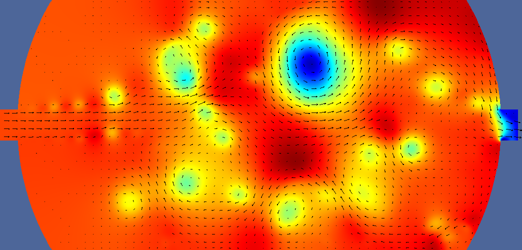
Pressure distribution after 105 seconds.
These runs use a fully mixed tracer, but the hypochlorite may not be fully mixed with the well water prior to entering the contact tank.
Unsteady conditions are taken as when the flow regime is forming in the tank. Tracer is introduced at 15 seconds into the simulation. After 115 seconds, turbulent flow has developed in the tank.
| condition | deltatime | Tracer | Vorticity | Velocity | Pressure |
|---|---|---|---|---|---|
| unsteady | 2 s |  | 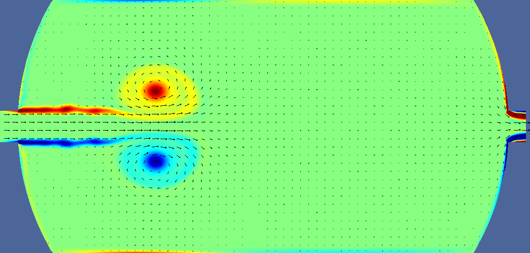 | ||
| unsteady | 17 s | 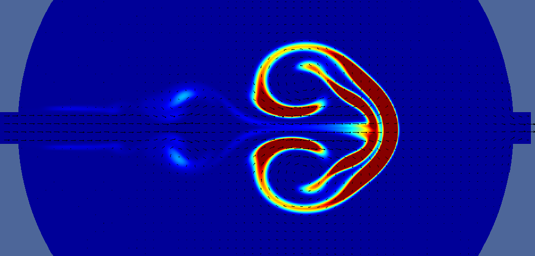 | 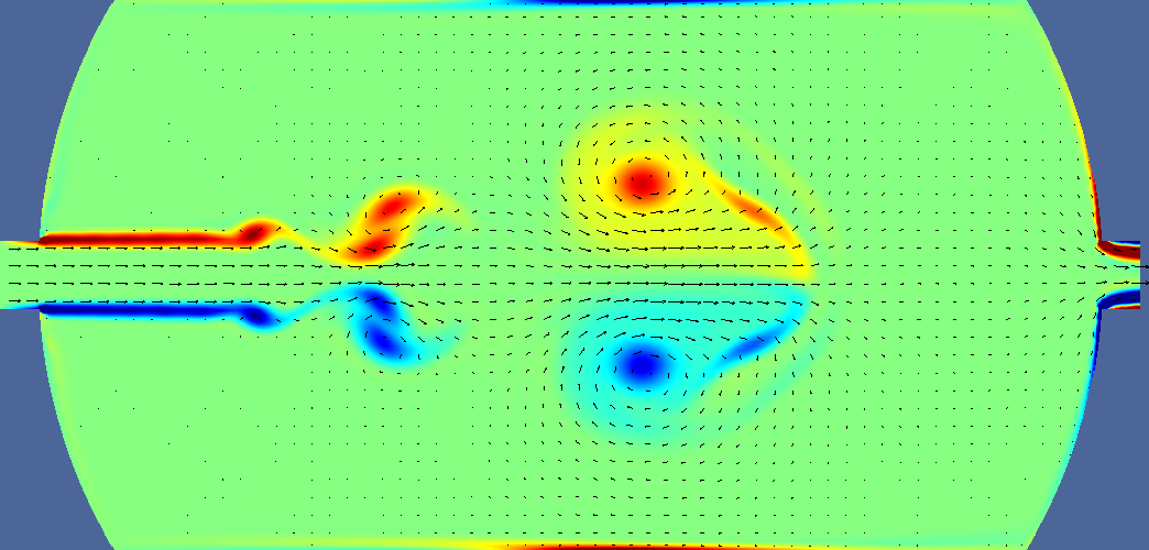 | 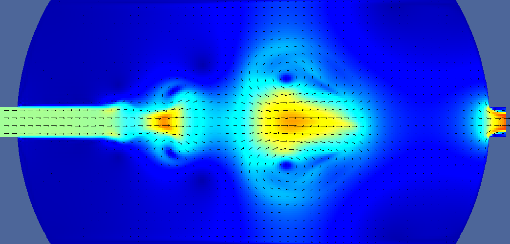 | |
| unsteady | 36 s |  | 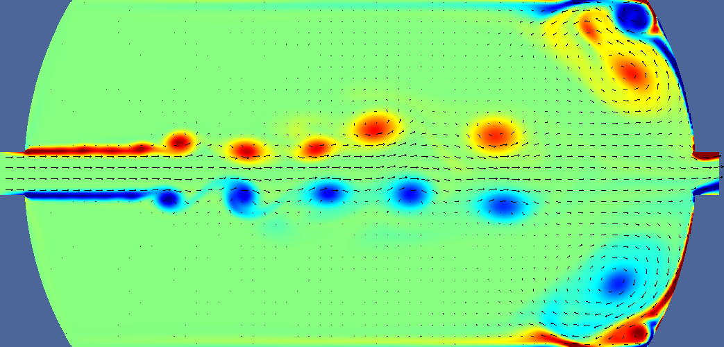 |  |  |
| steady | 4 s |  |  | ||
| steady | 16 s | 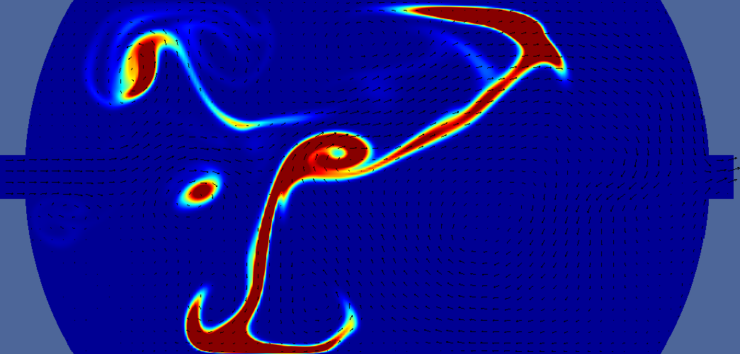 | 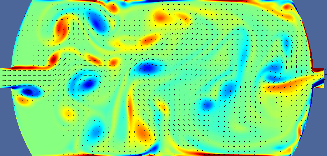 | ||
| steady | 35 s | 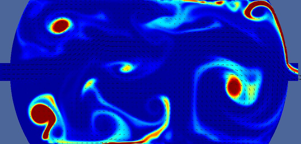 |  | ||
| steady baffle | 4 s |  | 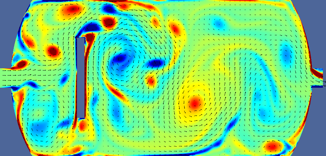 |  | |
| steady baffle | 16 s | 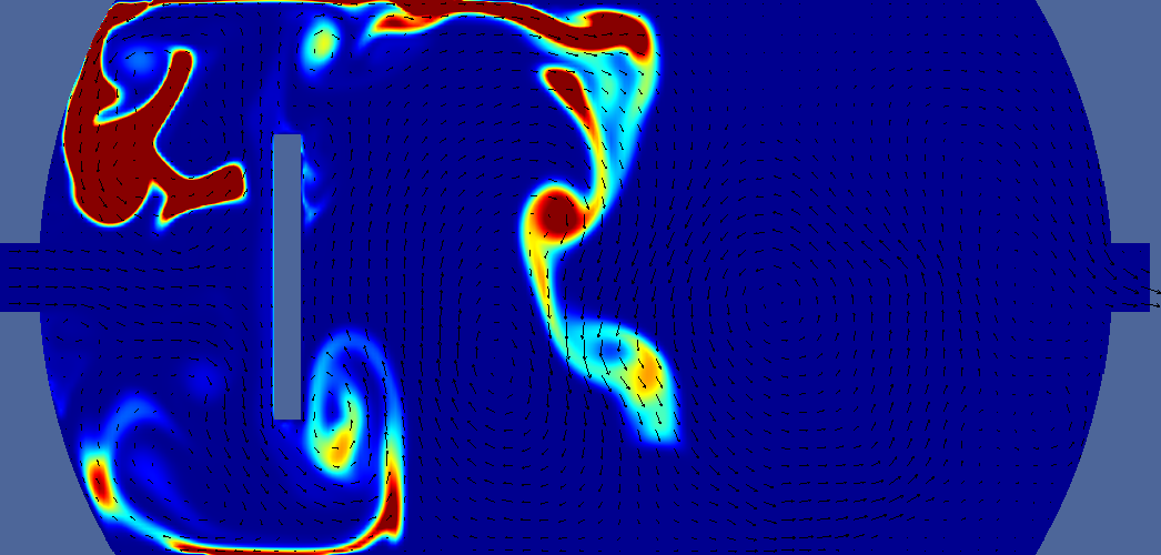 |  | ||
| steady baffle | 35 s |  | 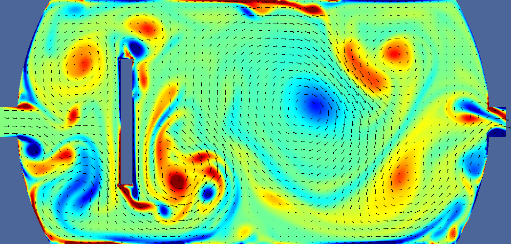 |  |
Deltatime is t-ttracer injection ends. For pressure, navy is minimum, burgundy is maximum. Light green is middle. For velocity navy is zero, burgundy is 0.2m/s, light green is 0.1 m/s. For vorticity navy is -5, burgundy is +5, light green is 0. For tracer navy is zero, burgundy is 0.05 (one twentieth of input concentration). Arrows indicate velocity direction and magnitude.
Steady Flow
Unsteady Flow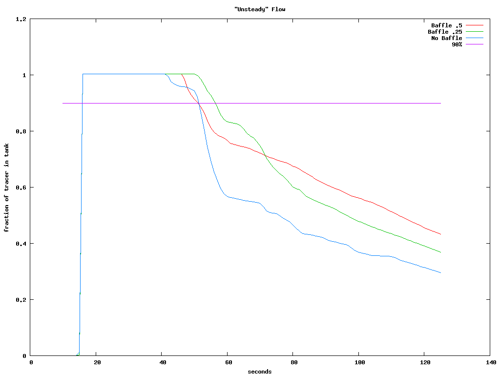
In these preliminary 2D tests, the baffle located at the one quarter point increased contact time compared to the baffle located in the middle or no baffle tanks. T10 is measured where tracer line crosses the 90% line.
| baffle | unsteady | steady |
|---|---|---|
| middle | 36 | 58 |
| .25 | 42 | 62 |
| none | 36 | 32 |
| baffle | unsteady | steady |
|---|---|---|
| middle | 29 | 25 |
| .25 | 34 | 26 |
| none | 26 | 23 |
Steady Flow, full graph
Three movies, the first two showing the velocity distribution in the unsteady .25 baffle run and unsteady .5 baffle run and the third showing tracer distribution in a test with input velocity ranging sinusoidally from 0.075 to 0.125 m/s./2/
Flow in contact tank takes time to form turbulence or stable condition/3/. Contact time can be reduced under these conditions. Unsteady conditions are the norm for small water plants since the chlorinator and well pump both turn on at the same time.
The Reynolds number in the inlet is near critical for turbulence. The Re in the tank is above critical for turbulence.
Transition from still to flowing conditions takes time. How long to stable? Check Re.
Initial momemtum carries tracer quickly across tank. Baffle increases path but also breaks up forward momentum of input water. Baffle closer to inlet improves retention by stopping input momemtum faster. As turbulent flow develops, initial momentum is also broken up, but partially mixed conditions exist.
At 0.1 m/s and 2 m long tank, tracer would take 20 seconds to cross tank with no baffle and no flow spreading. Moving the baffle from the middle to the first quarter reduces the distance from the inlet to the baffle 0.5 m or 5 seconds, which is what the model shows for initial (non turbulent) conditions.
Many existing detention tanks are mounted vertically. The inlet is on top, but the outlet is on the side of the bottom. Such an arrangement should not significantly change these results.
Sinusoidal input flow
Some contact tanks do not receive a steady incoming flow. Contact tanks positioned after hydropneumatic tanks have flow which varies with customer usage. Non steady input will change the flow characteristics in the tank.
Test results for non steady input.
Sinusoidal input flow
When tracer was injected as the velocity was increasing, T10 was 13 seconds, much lower than for steady input velocity. A second run with the opposite phase gave T10 in 33 seconds. For the second run the initial velocity when the tracer was injected was below average rather than above. The period of the flow oscillation is 31 seconds, so synchronization with the injection is very important. Still, nonsteady input velocity seems to decrease T10.
Sinusoidal input flow
Tests with a more stabilized
flow continue to show a variability in T10 based on when in the velocity cycle the tracer is injected. For these runs the sum of velocity (no units) across the entire tank was recorded. The velocity in the tank should reach a constant average since the input velocity has a constant average. The initial velocity in the tank is zero. That the average velocity in the tank has not stabilized within 150 seconds is troubling for contact tanks fed by pumps on short cycles. The rule of thumb for small motors (< 700 watts) is a minimum run time of 60 seconds. Turbulent conditions in the tank substantial (>10 percent) amounts of tracer to short circuit to the outlet.
The design of contact tanks usually assumes a peak flow for a period of 30 minutes or 2 hours. Higher flows might certainly be present for shorter time scales.
Contact tanks are designed to handle peak flows. During peak flow, turbulent conditions prevail in the tank. During average or off-peak, lower tank flows may produce laminar conditions. Although the theoretical contact time increases, so also may short circuiting.
Test results for .5 and .1 peak flow.
Diffusion may also have an effect on retention.
2D calcs. Note that in 2D area (A) is linear, Volume (V) is areal, etc.
Q = Av
  = (.12 m)(.1 m/s)
  = .012 m^2/s

V from simulation
1.728263 w/o baffle
1.703	 w/baffle
t = V/Q  'Plug flow contact time
  = (1.728 m^2)/(.012 m^2/s)
  = 144 s
  = 142 s

T10/T min = (32 s)/(144 s)
       = 0.22
T10/T max = (62 s)/(144 s)
             = 0.43
These ratios are better than the standard values, but the absolute times are too quick.
Reworking as 3D
1m diam x 1.8m cylinder = about 1400 liters
1m/s x .12 m diam pipe

Q = Av
(* .06 .06 3.14159 1)
0.011309723999999998 m^3/s Q
or 0.0011 for 0.1 m/s velocity

Volume
(* .5 .5 3.14159 1.8)
1.4137155 m^3 V

Plug Flow Contact time
Q=V/t or V/Q=t
(/ 1.4137155 0.011309723999999998)
125.00000000000001 s time
2 minutes
or 20 minutes for .1 m/s
Twenty minutes is a reasonable contact time. Thirty two to sixty two seconds T10 equates to T10/T of 0.025 to 0.05, which are somewhat below the rule of thumb values.
Reynolds number calculations.
ν or kinematic fluid viscosity of water at 10 deg C = 1.307 m^2/s x 10^(-6)
nu = 1.307 E-6 at 10 deg C
Re = v * cl / ν

For the inlet cl = 0.12 meters
(/ (* 1 .12) .000001307)
91813.
or 9181 for velocity of 0.1 m/s
For the tank cl = .95 meters
(/ (* .1 .95) .000001307)
or 72685 for velocity of 0.1 m/s

model viscosity = model velocity * real viscosity / real velocity * model length / real length
mnu = rnu(mv/rv)(ml/rl)
 mnu = .0000013 * 1/.1 * .12/.12
 = .000013
The simulations were run with input velocity of 0.1 m/s and kinematic viscosity 1 E-6 rather than unitizing and adjusting similitudes.
Dynamic refinement of the mesh produced less accurate results than fixed meshes and was abandoned for 2D work.
NYSDOH EHM Item PWS-41
USEPA guidance manuals
http://en.wikipedia.org/wiki/Continuous_stirred-tank_reactor
Simulation input files
/1/ This table is quoted all over, but rarely attributed.
/2/ Movies are in mpeg4 format. Use mplayer or ffmpeg/libavcodec.
/3/ Describing turbulent flow as steady is somewhat of an oxymoron.